
Life is messy, isn’t it? Things like tracking finances and managing time are messy and time-consuming. Yet, these are things that, if put in order, would improve your life. Spreadsheets can help every day with these sorts of tasks.
It can be challenging to find information in spreadsheets, however. That’s why we’re going to show you how to use the VLOOKUP function in Google Sheets to make finding something in a spreadsheet a lot easier.

VLOOKUP is a Sheets function to find something in the first column of a spreadsheet. The V is for vertical because, like columns on a building, spreadsheet columns are vertical. So when VLOOKUP finds the key thing we’re looking for, it will tell us the value of a specific cell in that row.
The VLOOKUP Function Explained
In the image below is the VLOOKUP function’s syntax. This is how the function is laid out, regardless of where it’s being used.

The function is the =VLOOKUP( ) part. Inside the function are:
- Search Key – Tells VLOOKUP what it needs to find.
- Range – Tells VLOOKUP where to look for it. VLOOKUP will always look in the leftmost column of the range.
- Index – Tells VLOOKUP how many columns to the right of the left-most column in the range to look for a value if it finds a match of the search key. The left-most column is always 1, the next to its right is 2, and so on.
- Is sorted? – Tells VLOOKUP if the first column is sorted. This defaults to TRUE, which means VLOOKUP will find the nearest match to the search key. This can lead to less accurate results. FALSE tells VLOOKUP that it must be an exact match, so use FALSE.
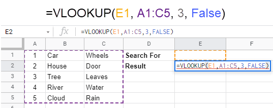
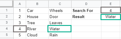
The VLOOKUP function above will use whatever value is in cell E1 as its search key. When it finds a match in column A of the range of cells from A1 to C5, it will look in the third column of the same row as it found the match and return whatever value is in it. The image below shows the results of entering 4 in cell E1. Next, let’s look at a couple of ways to use the VLOOKUP function in Google Sheets.
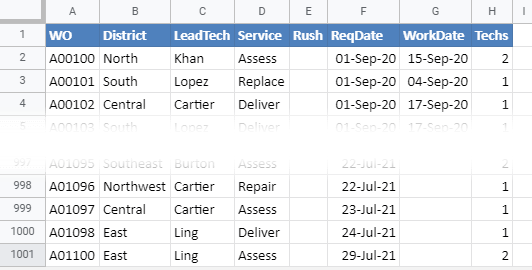
Example 1: Using VLOOKUP For Tracking Jobs
Let’s say you have a service business and you want to find out when a work order starts. You could have a single worksheet, scroll down to the work order number and then look across the row to find out when it starts. That can become tedious and prone to error.
Or you could use VLOOKUP.
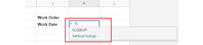
- Enter the headings Work Order and Work Date somewhere on the worksheet.

- Select the cell to the right of Work Date and start entering the formula =VLOOKUP. A help box will pop up as we type, showing us available Google Sheet functions that match what we’re typing. When it shows VLOOKUP, press Enter, and it will complete the typing.
- To set where VLOOKUP will find the Search Key, click on the cell right above this.

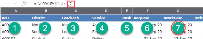
- To select the Range of data to search in, click and hold on the A column header and drag to select everything over to, including column H.

- To select the Index, or column, that we want to pull data from, count from A to H. H is the 7th column so enter 7 in the formula.
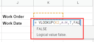
- Now we state how we want the first column of the range to be searched. We need an exact match so enter FALSE.
Notice that it wants to put an opening curved bracket after FALSE. Press backspace to remove that.
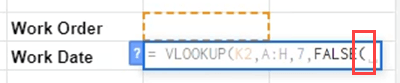
Then enter a curved closing bracket ), and press Enter to finish the formula.

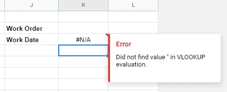
We’ll see an error message. That’s ok; we did things correctly. The issue is that we don’t have a search key value yet.
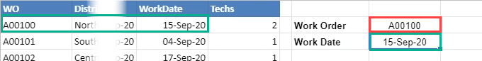
To test the VLOOKUP formula, enter the first work order number in the cell above the formula and press Enter. The date returned matches the date in the WorkDate column for work order A00100.
To see how this makes life easier, enter a work order number that isn’t visible on the screen, like A00231.
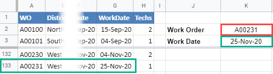
Compare the date returned and the date in the row for A00231, and they should match. If they do, the formula is good.
Example 2: Using VLOOKUP to Calculate Daily Calories
The Work Order example is good but simple. Let’s see the actual power of VLOOKUP in Google Sheets by creating a daily calorie calculator. We’ll put the data in one worksheet and make the calorie calculator in another.
- Select all the data on the food and calorie list.

- Select Data > Named Ranges.
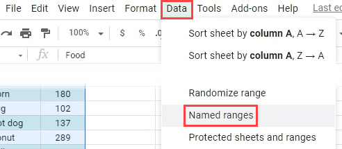
- Name the range FoodRange. Named ranges are easier to remember than Sheet2!A1:B:29, which is the actual definition of the range.

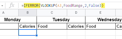
- Go back to the worksheet where food is tracked. In the first cell in which we want calories to show, we could enter the formula =VLOOKUP(A3,FoodRange,2,False).
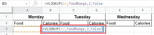
It would work, but because there’s nothing in A3, there will be an ugly #REF error. This calculator might have many Food cells left blank and we don’t want to see #REF all over it.
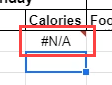
- Let’s put the VLOOKUP formula inside an IFERROR function. IFERROR tells Sheets that if anything goes wrong with the formula, return a blank.
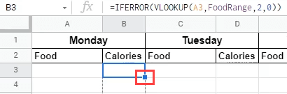
- To copy the formula down the column, select the handle at the bottom-right corner of the cell and drag it down over as many cells as needed.
If you think that the formula will use A3 as the key down the column, don’t worry. Sheets will adjust the formula to use the key in the row that the formula is in. For example, in the image below, you can see that the key changed to A4 when moved to the 4th row. Formulas will automatically change cell references like this when moved from column to column, too.

- To add up all the calories in a day, use the =SUM function in the blank cell next to Total, and select all the rows of calories above it.
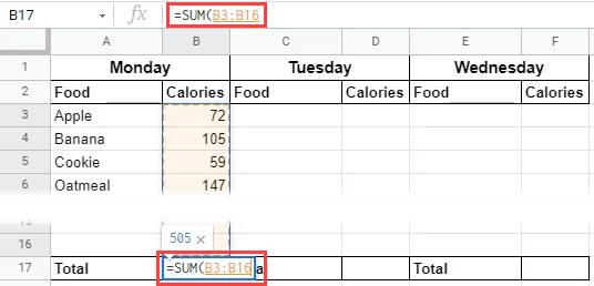
Now we can see how many calories we had today.
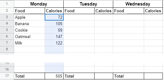
- Select the column of calories from Monday and paste it to the Calories column for Tuesday, Wednesday, and so on.

Do the same for the Total cell below Monday. So now we have a weekly calorie counter.

Summing Up VLOOKUP
If this is your first dive into Google Sheets and functions, you can see how useful and powerful functions like VLOOKUP can be. Combining it with other functions like IFERROR, or so many others, will help you do whatever you need. If you enjoyed this, you might even consider converting from Excel to Google Sheets.
source https://www.online-tech-tips.com/computer-tips/how-to-use-vlookup-in-google-sheets/